Can a Machine Learn to Be a Firewall? Classifying Internet Traffic with Data Science
Introduction
Every second, your internet connection is handling thousands of tiny digital conversations — loading web pages, sending emails, streaming videos, and more. Sitting between you and the vast internet is a firewall: a digital gatekeeper that decides which of those conversations are safe to let through and which should be blocked.
But what if we could teach a computer to learn the patterns behind those decisions? That is exactly what this project explores. Using a real-world dataset of over 65,000 internet traffic log entries, we built machine learning models that can classify network traffic into one of four firewall actions — Allow, Deny, Drop, or Reset — with remarkable accuracy.
In this post, we walk through the entire journey: understanding the data, cleaning it up, exploring interesting patterns, and finally training two powerful machine learning models to make predictions.
The Data: What Does Internet Traffic Look Like?
The dataset (log2.csv) contains 65,532 records of network traffic captured by a firewall. Each record has 12 columns — 11 input features describing the traffic and 1 target label indicating the firewall’s decision.
Here is a quick look at what each feature represents:
| Feature | What It Means |
|---|---|
| Source Port | The “door number” on the sender’s computer |
| Destination Port | The “door number” on the receiver’s computer |
| NAT Source Port | The translated sender port (after Network Address Translation) |
| NAT Destination Port | The translated receiver port |
| Bytes | Total data transferred |
| Bytes Sent | Data sent by the source |
| Bytes Received | Data received by the source |
| Packets | Total number of data packets |
| Elapsed Time (sec) | How long the connection lasted |
| pkts_sent | Number of packets sent |
| pkts_received | Number of packets received |
| Action | The firewall’s decision: allow, deny, drop, or reset-both |
Think of ports as apartment numbers in a building. When your computer sends data, it picks a “door” to send from (source port) and addresses it to a specific “door” on the receiving machine (destination port). Common doors you might recognize: port 80 is for regular web traffic (HTTP), port 443 is for secure web traffic (HTTPS), and port 53 is for DNS lookups (translating website names like “google.com” into numeric addresses).
One important note: the dataset has no missing values, which means every record is complete — a luxury in the data science world!
Data Preview
Below is a scrollable preview showing the structure of the dataset. Each row represents one network connection captured by the firewall.
⬇ Download the full dataset from Kaggle
| Source Port | Destination Port | NAT Source Port | NAT Destination Port | Bytes | Bytes Sent | Bytes Received | Packets | Elapsed Time (sec) | pkts_sent | pkts_received | Action |
|---|---|---|---|---|---|---|---|---|---|---|---|
| 57222 | 53 | 57222 | 53 | 186 | 119 | 67 | 2 | 0 | 1 | 1 | allow |
| 54487 | 443 | 54487 | 443 | 2870 | 1370 | 1500 | 7 | 1 | 4 | 3 | allow |
| 46498 | 80 | 0 | 0 | 0 | 0 | 0 | 1 | 0 | 1 | 0 | deny |
| 62092 | 443 | 0 | 0 | 0 | 0 | 0 | 1 | 0 | 1 | 0 | drop |
| 51773 | 443 | 51773 | 443 | 15422 | 4082 | 11340 | 18 | 3 | 8 | 10 | allow |
Showing 5 representative rows of 65,532 total × 12 columns, illustrating allow, deny, and drop actions.
Exploring the Data: What Can We See?
How Does the Firewall Usually Respond?
The first thing we want to know is: how often does the firewall allow traffic versus block it?
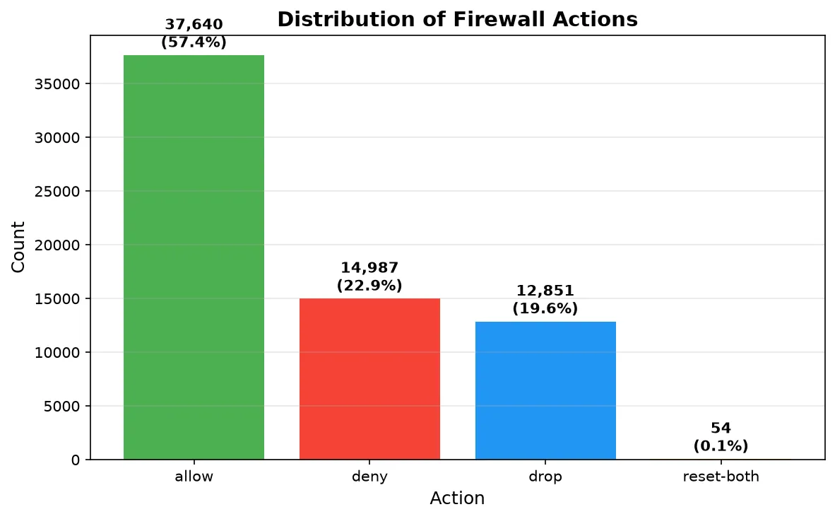
The answer reveals an imbalanced dataset:
- Allow: ~37,640 records (57.4%) — the majority of traffic is permitted
- Deny: ~14,987 records (22.9%) — actively refused
- Drop: ~12,851 records (19.6%) — silently discarded
- Reset-both: only 54 records (0.08%) — extremely rare
This imbalance is important because machine learning models can struggle with very rare categories. The “reset-both” class, with only 54 examples out of 65,000+, is particularly challenging — imagine trying to learn what a rare bird looks like when you have only seen it a handful of times.
Which Ports Are Most Popular?
Next, we examined which ports appear most frequently. This tells us what kinds of internet traffic dominate the dataset.
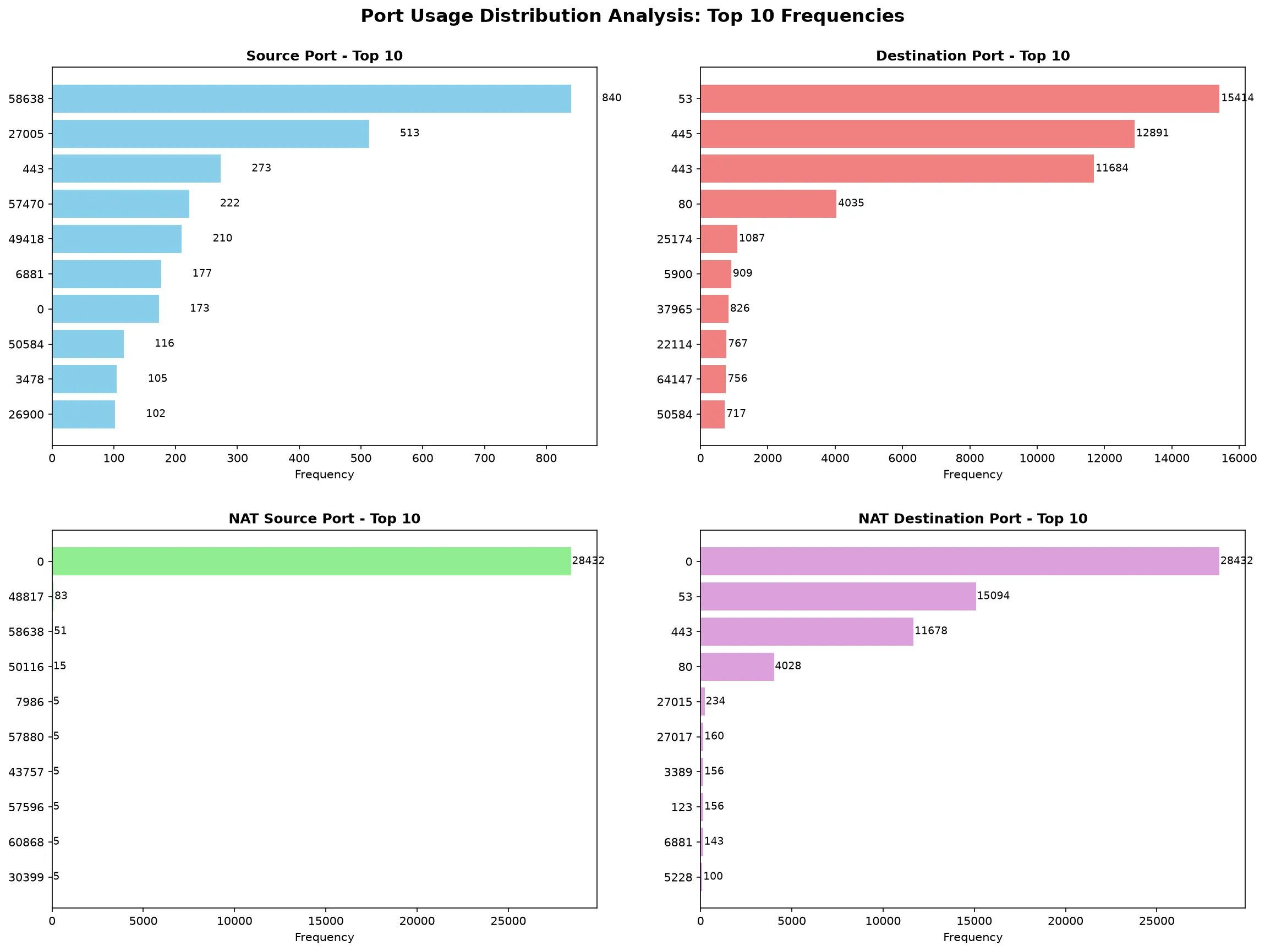
Key observations:
- Destination ports 53, 443, and 80 dominate — these correspond to DNS, HTTPS, and HTTP traffic. In other words, most connections are simply web browsing and name resolution.
- Port 0 appears frequently in the NAT (translated) ports. Port 0 is not a real port — it is a placeholder, often indicating that no translation was needed or the connection was blocked before translation occurred.
- The source ports are much more varied, as computers typically pick random high-numbered ports for outgoing connections.
How Are the Numerical Features Related?
We also examined how the numerical features relate to each other using a correlation heatmap:
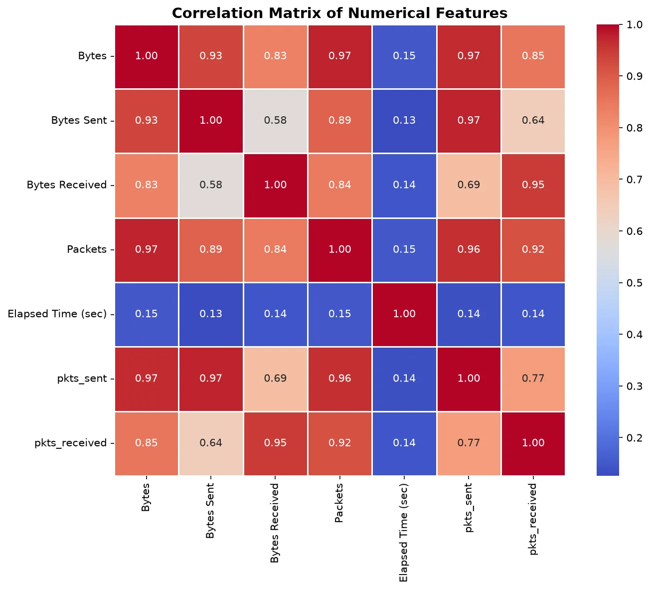
The heatmap reveals something important: several features are extremely correlated with each other. For example:
- Bytes = Bytes Sent + Bytes Received (they are mathematically linked)
- Packets = pkts_sent + pkts_received (same relationship)
When features are this tightly linked, it creates a problem called multicollinearity — essentially, the model receives the same information multiple times, which can confuse it. We confirmed this using a statistical measure called the Variance Inflation Factor (VIF), which showed astronomically high values for the redundant features.
The solution? We kept only the component features (Bytes Sent, Bytes Received, pkts_sent, pkts_received, and Elapsed Time) and dropped the totals (Bytes and Packets). This gives the model the same information without the redundancy.
Preparing the Data for Machine Learning
Before feeding data into a model, we need to transform it into a format that algorithms can understand.
Handling Port Numbers: Top-N Encoding
Port numbers might look like regular numbers, but they are actually categories — port 443 is not “bigger” or “better” than port 80; they just represent different types of services. This means we need to use a technique called One-Hot Encoding (OHE), which creates a separate yes/no column for each unique port value.
The problem? Source Port alone has over 22,000 unique values. Creating 22,000+ columns would make the dataset enormous and the model extremely slow.
The clever solution is Top-N Encoding: we keep only the most frequently occurring port values and group everything else into an “Other” category. In this project, we retained the top 1% of port values by frequency. This reduced thousands of unique ports into a manageable number while preserving the most important information.
After this encoding, we ended up with approximately 580 features — still a lot, but manageable.
Scaling Numerical Features
Machine learning models work best when numerical features are on similar scales. A feature like “Bytes Sent” can range from 0 to millions, while “pkts_sent” might only go from 0 to a few hundred. We used Standard Scaling (subtracting the mean and dividing by the standard deviation) to put all numerical features on equal footing.
Building the Models
With our data prepared (about 580 features, 65,000+ records, split 80/20 into training and test sets), we trained two different machine learning models.
Model 1: Support Vector Machine (SVM)
A Support Vector Machine is a classic machine learning algorithm that works by finding the best “boundary” to separate different classes. Think of it like drawing lines on a map to separate countries — SVM finds the lines that create the widest possible buffer zones between groups.
We used a linear SVM (meaning it draws straight lines rather than curves) with a regularization parameter C = 1. Despite the simplicity of a straight-line approach, the results were impressive:
SVM Test Accuracy: 99.66%
We also tested different values of the regularization parameter C (from 0.001 to 1000) using cross-validation — a technique that trains and tests the model on different portions of the data to ensure the results are reliable. The accuracy remained consistently above 99% across all settings.
However, SVM has a downside: it is computationally expensive for large datasets. With 580 features and 65,000 records, training took a significant amount of time.
Model 2: Stochastic Gradient Descent (SGD)
Stochastic Gradient Descent is a much faster alternative. Instead of looking at all the data at once (like SVM does), SGD processes small random batches of data and gradually improves its predictions. This makes it much more practical for larger datasets.
We configured SGD with a log loss function (making it behave similarly to logistic regression) and early stopping (automatically stopping when further training stops improving results).
SGD Test Accuracy: 99.57%
Nearly identical to SVM — and it trained much faster.
Comparing the Models: ROC Curves
To get a deeper understanding of how well each model performs, we looked at ROC curves (Receiver Operating Characteristic curves). These plots show how well a model distinguishes between classes at different confidence thresholds.
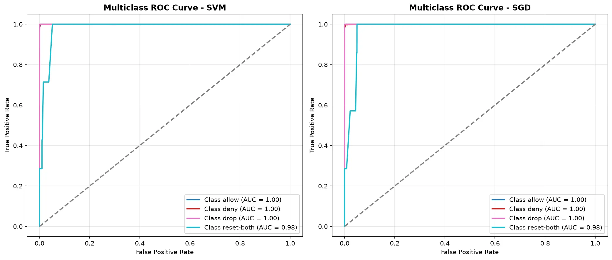
The closer a curve hugs the top-left corner, the better the model is at separating that class from the others. A perfect classifier would have an AUC (Area Under the Curve) of 1.00.
Both models achieved near-perfect AUC scores for the Allow, Deny, and Drop classes. The only weakness? The reset-both class, which had too few examples (only 7 in the test set) for either model to learn effectively.
Detailed Performance Breakdown
| Class | SVM Precision | SVM Recall | SGD Precision | SGD Recall |
|---|---|---|---|---|
| Allow | 1.00 | 1.00 | 1.00 | 1.00 |
| Deny | 1.00 | 0.99 | 0.99 | 1.00 |
| Drop | 1.00 | 1.00 | 1.00 | 1.00 |
| Reset-both | 0.00 | 0.00 | 0.00 | 0.00 |
Both models essentially perform identically on the three main classes. Neither model could learn the “reset-both” pattern due to the extreme scarcity of examples — this is a classic challenge in machine learning known as the class imbalance problem.
Key Takeaways
-
Firewall decisions are highly learnable. With the right features and preprocessing, machine learning models can classify network traffic with over 99.5% accuracy.
-
Feature engineering matters. Ports are categories, not numbers. Using Top-N encoding to handle high-cardinality categorical features and removing redundant numerical features (via VIF analysis) were critical steps.
-
Simpler models can be just as good. The linear SVM and SGD models — both essentially drawing straight-line boundaries — achieved nearly perfect accuracy. There was no need for complex nonlinear models.
-
Speed versus accuracy is a real trade-off. SVM was marginally more accurate but took much longer to train. SGD delivered nearly the same performance in a fraction of the time, making it the more practical choice for large-scale applications.
-
Rare events are hard to predict. The “reset-both” class, comprising less than 0.1% of the data, was effectively invisible to both models. In real-world applications, techniques like oversampling, SMOTE, or cost-sensitive learning could help address this.
Conclusion
This project demonstrates that data science can be a powerful ally in cybersecurity. By analyzing patterns in internet traffic logs, we can build models that classify firewall actions with remarkable precision. While these models are not a replacement for carefully configured firewall rules, they show the potential for automated threat detection and anomaly identification in network security.
The next time your web page loads smoothly or a suspicious connection gets blocked, remember — behind the scenes, decisions like these are happening thousands of times per second. And as this project shows, machines can learn to make those decisions almost as well as the rules written by human experts.