Predicting Company Bankruptcy with Machine Learning: A Comparative Study of Random Forest and XGBoost
Introduction
Can we predict whether a company is heading toward bankruptcy before it actually happens? This question is important for investors, banks, regulators, and employees alike. If we could identify warning signs early enough, stakeholders could take action—whether that means restructuring the business, adjusting investment portfolios, or tightening lending criteria.
In this post, we walk through a machine learning project that attempts to answer exactly that question. Using financial data from Polish companies, we build and compare two popular classification algorithms—Random Forest and XGBoost—to see how well they can distinguish bankrupt firms from healthy ones. Along the way, we explore data cleaning, feature selection, and model evaluation techniques that are foundational to any data science workflow.
The Dataset
The data comes from the Polish Companies Bankruptcy dataset, originally hosted on the UCI Machine Learning Repository. It contains financial ratios computed from annual reports of Polish companies, spanning five time windows (Year 1 through Year 5). Each record represents one company in one year and includes:
- 64 financial ratio features (labeled X1 through X64), such as net profit to total assets, total liabilities to total assets, and working capital to total assets.
- A bankruptcy label (1 = bankrupt, 0 = not bankrupt).
- A year indicator (1 through 5).
After merging all five files, the combined dataset contains 43,405 records. Only 2,091 of these (about 4.8%) are bankrupt companies—making this a classic example of an imbalanced classification problem, where one class is far more common than the other.
Data Preview
Below is a scrollable preview showing the structure of the merged dataset. Each row represents one company in one year, with 64 financial ratio features (X1–X64), a bankruptcy label (class), and a year indicator.
⬇ Download the full dataset from UCI Machine Learning Repository
| X1 | X2 | X3 | X4 | X5 | ... | X62 | X63 | X64 | class | year |
|---|---|---|---|---|---|---|---|---|---|---|
| 0.1740 | 0.4047 | 0.2286 | 0.1578 | 0.3550 | ... | 0.1115 | 0.0369 | 0.0702 | 0 | 1 |
| 0.1460 | 0.3565 | 0.2032 | 0.1244 | 0.4102 | ... | 0.0978 | 0.0244 | 0.0610 | 0 | 1 |
| 0.0921 | 0.2212 | 0.1099 | 0.0855 | 0.5134 | ... | 0.0587 | 0.0151 | 0.0413 | 1 | 3 |
Showing 3 representative rows of 43,405 total × 66 columns (64 features + class + year). Columns X6–X61 omitted for display.
Data Cleaning and Preprocessing
Handling Missing Values
Real-world data is rarely perfect, and this dataset is no exception. Our first step was to examine how much data was missing across each feature.
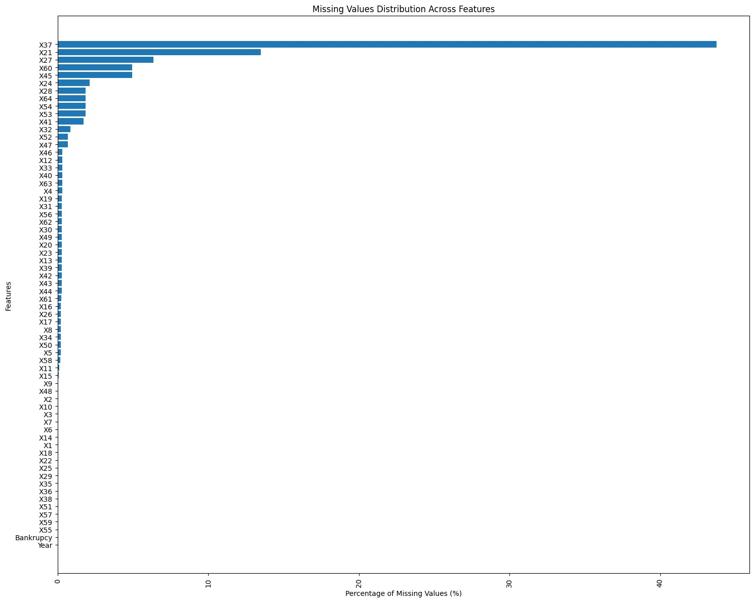 Figure 1: Percentage of missing values for each feature. X37 stands out with nearly 44% of its values missing.
Feature X37 (representing the ratio of current assets minus inventories to long-term liabilities) had an exceptionally high percentage of missing data—nearly 44%. Because so much of this feature’s information was absent and other related variables in the dataset could capture similar financial signals, we decided to remove X37 entirely rather than attempt to impute nearly half its values.
For the remaining features, missing values were filled in using a technique called KNN Imputation (K-Nearest Neighbors Imputation with k=5). The basic idea is intuitive: for each company with a missing value, the algorithm looks at the five most similar companies (based on the features that are available) and fills in the gap using the average of their values. This is generally more reliable than simply plugging in the overall column average, because it accounts for the relationships between features.
After cleaning, we were left with 63 features and no missing values.
Exploratory Data Analysis
Bankruptcy Rates by Year
Before diving into modeling, it helps to understand the data. We first looked at how the bankruptcy rate varies across the five year-windows.
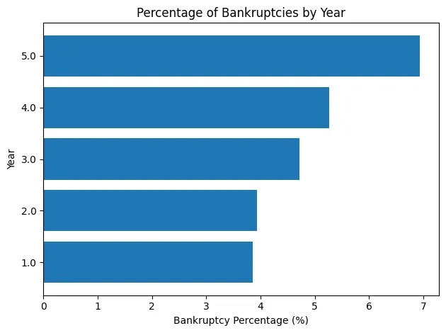 Figure 2: Bankruptcy rates by year. Companies closer to the point of failure (Year 5) show higher bankruptcy percentages (~7%) compared to those further away (Year 1, ~4%).
An interesting pattern emerges: the bankruptcy percentage increases as we move from Year 1 to Year 5. Year 5 has the highest rate at around 7%, while Year 1 sits near 4%. This makes intuitive sense—companies closer to their eventual failure date are more likely to already be exhibiting signs of financial distress in their annual reports.
Understanding Feature Relationships with Clustering
With 63 features, it is natural to ask: Are some of these features measuring the same underlying financial health signal? To answer this, we computed the cross-correlation matrix—a table showing how strongly every pair of features moves together—and applied hierarchical clustering to group similar features.
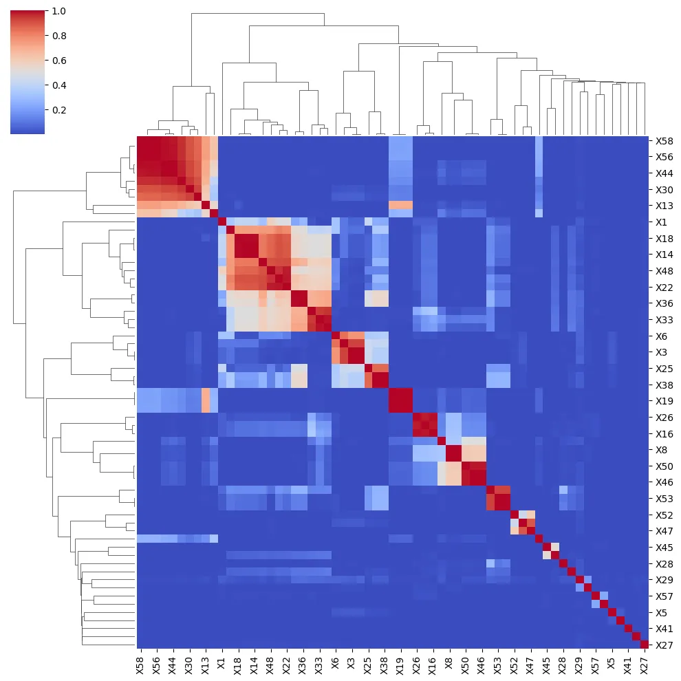 Figure 3: A clustered heatmap of cross-correlations among all 63 features. Dark red indicates strong positive correlation; dark blue indicates weak or no correlation. Dendrograms on the sides show how features group together.
This visualization reveals clear structure in the data. One prominent cluster (the bright red block in the upper-left) contains features that are highly correlated with each other—essentially measuring similar aspects of a company’s financial condition.
Zooming into the Dominant Cluster
We identified the largest cluster (Cluster ID 8) and inspected its features more closely:
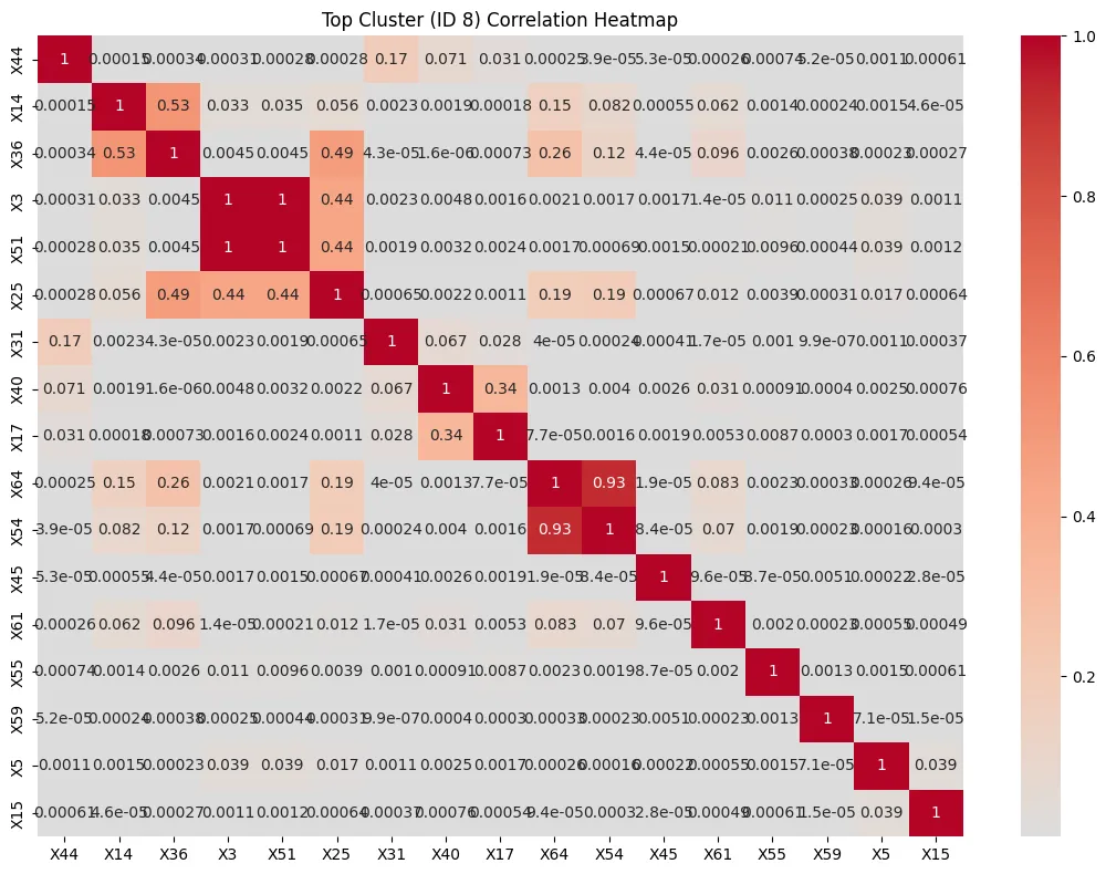 Figure 4: Detailed correlation heatmap for the 17 features in the top cluster. Notable pairs like X64/X54 (r = 0.93) and X3/X51 (r = 1.0) indicate near-duplicate information.
This cluster contained 17 features: X44, X14, X36, X3, X51, X25, X31, X40, X17, X64, X54, X45, X61, X55, X59, X5, and X15. Several pairs showed extremely high correlations—for instance, X3 and X51 had a correlation of essentially 1.0 (they carry the same information), and X64 and X54 had a correlation of 0.93.
To create a reduced feature set, we kept this cluster’s features but removed X51 and X54 (the redundant halves of the two most correlated pairs), leaving us with 15 selected features. This “selected” dataset would allow us to test whether a smaller, more focused set of financial ratios could match the performance of the full 63-feature set.
Building the Models
We trained four models in total, using an 80/20 train-test split:
| Model | Algorithm | Features Used |
|---|---|---|
| RF Full | Random Forest | All 63 features |
| RF Selected | Random Forest | 15 selected features |
| XGB Full | XGBoost | All 63 features |
| XGB Selected | XGBoost | 15 selected features |
What Are Random Forest and XGBoost?
Random Forest (RF) builds many individual decision trees (100 in our case), each trained on a random subset of the data and features. The final prediction is determined by majority vote across all trees. This “wisdom of the crowd” approach tends to be robust and resistant to overfitting.
XGBoost (Extreme Gradient Boosting) takes a different approach. Instead of building trees independently, it builds them sequentially—each new tree specifically focuses on correcting the mistakes of the previous ones. This iterative refinement often yields higher accuracy, especially on structured/tabular data.
Results
Accuracy Can Be Misleading
At first glance, all four models appear to perform well:
| Model | Accuracy |
|---|---|
| RF Full | 96% |
| RF Selected | 95% |
| XGB Full | 97% |
| XGB Selected | 95% |
But here is the catch: because only ~5% of companies in the dataset are bankrupt, a naive model that always predicts “not bankrupt” would still achieve about 95% accuracy! This is the trap of imbalanced datasets—accuracy alone does not tell the whole story.
To truly evaluate how well each model identifies bankrupt companies, we need to look at metrics that focus specifically on the minority class (bankruptcy).
Classification Performance on Bankrupt Companies
| Model | Precision (Class 1) | Recall (Class 1) | F1-Score (Class 1) |
|---|---|---|---|
| RF Full | 0.56 | 0.07 | 0.12 |
| RF Selected | 0.05 | 0.01 | 0.01 |
| XGB Full | 0.89 | 0.36 | 0.52 |
| XGB Selected | 0.17 | 0.03 | 0.05 |
Here the picture changes dramatically:
- Precision answers: Of the companies the model flagged as bankrupt, how many actually were? XGB Full leads with 0.89—when it raises a red flag, it is almost always right.
- Recall answers: Of all the actually bankrupt companies, how many did the model catch? Even the best model (XGB Full at 0.36) misses the majority of bankrupt firms.
- F1-Score balances precision and recall. XGB Full’s 0.52 is the best, but still indicates room for improvement.
The selected-feature models (RF Selected and XGB Selected) performed substantially worse, suggesting that the features outside the dominant cluster still carry important predictive signals.
ROC Curves: The Big Picture
The Receiver Operating Characteristic (ROC) curve provides perhaps the clearest comparison. It plots the trade-off between catching true positives (actual bankruptcies correctly identified) and false positives (healthy companies mistakenly flagged). The Area Under the Curve (AUC) summarizes this trade-off in a single number—a perfect model scores 1.0, while random guessing scores 0.5.
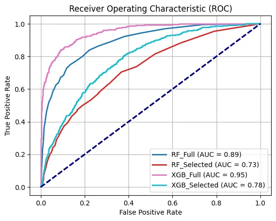 Figure 5: ROC curves comparing all four models. XGB Full (pink, AUC = 0.95) clearly outperforms the others, followed by RF Full (blue, AUC = 0.89). The dashed diagonal line represents random guessing.
The results are striking:
- XGB Full (AUC = 0.95) is the clear winner, demonstrating excellent ability to distinguish bankrupt from non-bankrupt companies.
- RF Full (AUC = 0.89) performs well but falls short of XGBoost.
- XGB Selected (AUC = 0.78) and RF Selected (AUC = 0.73) trail significantly, confirming that limiting features to the top cluster sacrifices predictive power.
What Features Matter Most?
We also examined which financial ratios each model relied on most heavily when making predictions.
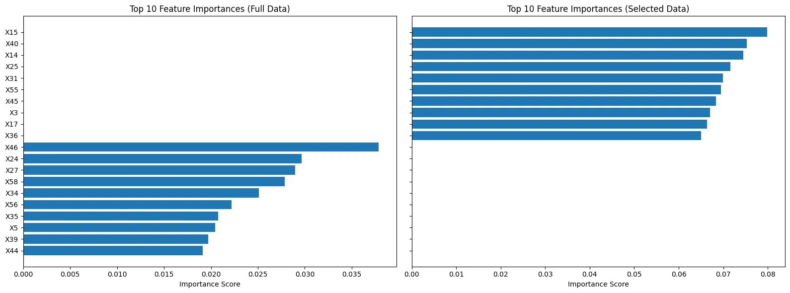 Figure 6: Top 10 most important features for Random Forest models. The full model (left) uses a diverse set of features, while the selected model (right) distributes importance more evenly among its 15 features.
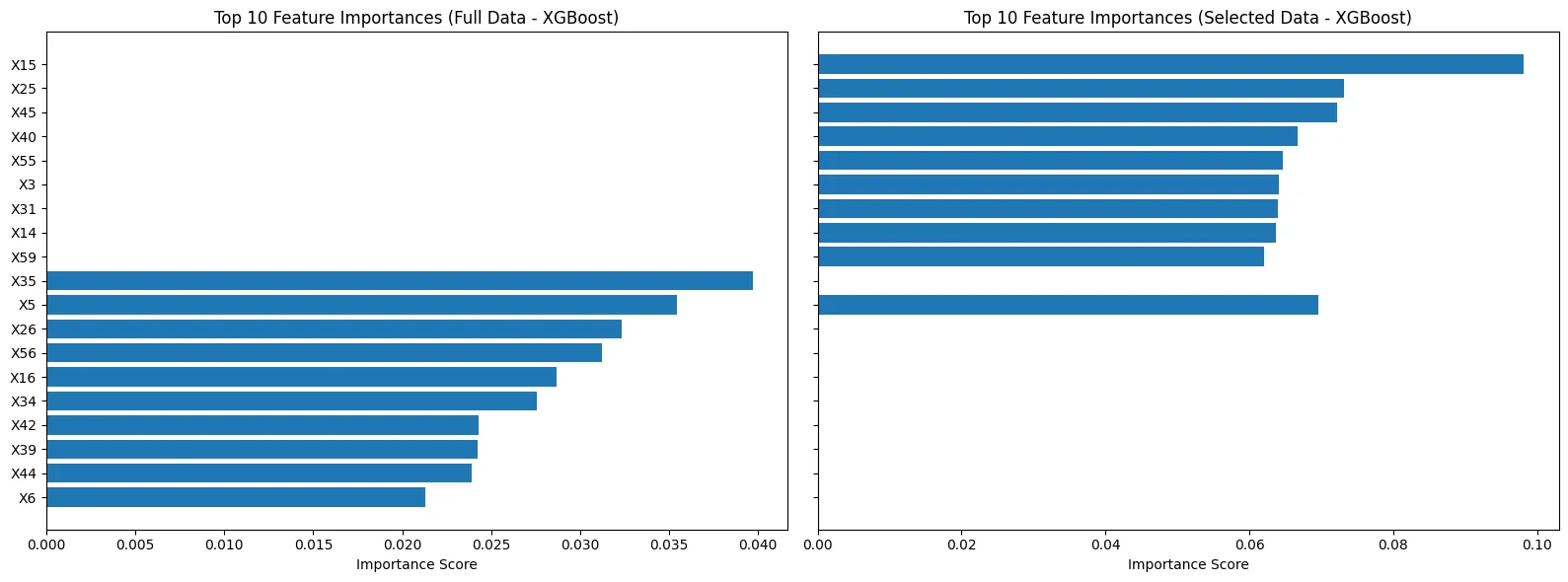 Figure 7: Top 10 most important features for XGBoost models. Similar pattern—the full model draws on a wider range of signals.
A few observations:
- X15 (short-term liabilities to total assets) appears as the top or near-top feature across multiple models, suggesting it is a particularly strong indicator of bankruptcy risk.
- The full models draw on a broader range of features, which likely explains their superior performance—they can detect subtler financial signals that the reduced feature set misses.
- The selected models spread importance more evenly among their 15 features, indicating that no single feature in the cluster dominates the prediction on its own.
Key Takeaways
-
XGBoost outperformed Random Forest on this bankruptcy prediction task, achieving the highest AUC (0.95) and the best precision-recall trade-off for identifying bankrupt companies.
-
More features helped. Despite the intuitive appeal of using a curated subset of highly correlated features, the full feature set consistently outperformed the selected subset across both algorithms. This suggests that the “less informative” features still contribute meaningful predictive signals when combined.
-
Accuracy is not enough. In imbalanced datasets, high accuracy can be deceptive. Metrics like AUC, precision, recall, and F1-score provide a much more honest assessment of model performance—especially for the minority class that we care about most.
-
Data quality matters. Thoughtful handling of missing values (removing X37, imputing the rest with KNN) and understanding feature relationships through correlation analysis laid the groundwork for effective modeling.
-
Even the best model has limitations. With a recall of 0.36, XGB Full catches only about one in three bankrupt companies. In a real-world application, further techniques such as class rebalancing (e.g., SMOTE), cost-sensitive learning, or threshold tuning could improve detection rates.
Conclusion
Predicting company bankruptcy from financial ratios is a challenging but valuable task. Our analysis shows that modern machine learning algorithms—particularly XGBoost—can extract meaningful patterns from financial data and provide strong discriminatory power (AUC = 0.95) between healthy and failing companies. However, the inherent class imbalance means that practitioners must go beyond simple accuracy and carefully tune their models to balance the trade-off between catching true bankruptcies and minimizing false alarms.
For anyone beginning their data science journey, this project illustrates several important lessons: always explore your data before modeling, understand the limitations of common metrics, and never underestimate the value of proper data preprocessing.
Data Source: Polish Companies Bankruptcy Data from the UCI Machine Learning Repository.