Predicting Superconductor Critical Temperature Using L1 and L2 Regularization
Introduction
Superconductors are materials that can conduct electricity with zero resistance when cooled below a characteristic temperature known as the critical temperature ((T_c)). Discovering new superconductors and predicting their critical temperatures is a central challenge in materials science, as higher (T_c) materials could revolutionize energy transmission, magnetic levitation, and quantum computing.
In this study, we explore whether the critical temperature of a superconductor can be accurately predicted from its elemental and physical properties using regularized linear regression. Specifically, we compare Ridge Regression (L2 regularization) and Lasso Regression (L1 regularization) — two powerful techniques that address multicollinearity and perform automatic feature selection.
The Dataset
The dataset used in this study comes from a publicly available superconductor dataset and consists of two files:
1. train.csv — Physical Property Features
| Property | Value |
|---|---|
| Samples | 21,263 superconductor compositions |
| Predictors | 81 features + 1 target |
| Target | critical_temp (in Kelvin) |
The 81 predictors are derived from 8 fundamental physical properties of the constituent elements:
- Atomic Mass
- First Ionization Energy (fie)
- Atomic Radius
- Density
- Electron Affinity
- Fusion Heat
- Thermal Conductivity
- Valence
Each property is summarized across the elements in a given compound using 10 statistical aggregation functions: mean, weighted mean, geometric mean, weighted geometric mean, entropy, weighted entropy, range, weighted range, standard deviation, and weighted standard deviation. Together with number_of_elements, this yields 81 predictors.
2. unique_m.csv — Elemental Composition Features
This supplementary file contains 86 columns corresponding to individual chemical elements (H, He, Li, …, Rn), each representing the proportion or count of that element in the compound. It also includes the critical_temp target and a material column with the chemical formula (e.g., Ba0.2La1.8Cu1O4).
Target Variable Summary
| Statistic | Value |
|---|---|
| Mean | 34.42 K |
| Std. Dev. | 34.25 K |
| Min | 0.00021 K |
| 25th Percentile | 5.37 K |
| Median | 20.00 K |
| 75th Percentile | 63.00 K |
| Max | 185.00 K |
Data Preview
Below is a scrollable preview of the first 3 rows of train.csv (out of 21,263). Scroll horizontally to see all 82 columns.
⬇ Download the full dataset (superconductor_data.tar.gz)
| number_of_elements | mean_atomic_mass | wtd_mean_atomic_mass | gmean_atomic_mass | wtd_gmean_atomic_mass | entropy_atomic_mass | wtd_entropy_atomic_mass | range_atomic_mass | wtd_range_atomic_mass | std_atomic_mass | wtd_std_atomic_mass | mean_fie | wtd_mean_fie | gmean_fie | wtd_gmean_fie | entropy_fie | wtd_entropy_fie | range_fie | wtd_range_fie | std_fie | wtd_std_fie | mean_atomic_radius | wtd_mean_atomic_radius | gmean_atomic_radius | wtd_gmean_atomic_radius | entropy_atomic_radius | wtd_entropy_atomic_radius | range_atomic_radius | wtd_range_atomic_radius | std_atomic_radius | wtd_std_atomic_radius | mean_Density | wtd_mean_Density | gmean_Density | wtd_gmean_Density | entropy_Density | wtd_entropy_Density | range_Density | wtd_range_Density | std_Density | wtd_std_Density | mean_ElectronAffinity | wtd_mean_ElectronAffinity | gmean_ElectronAffinity | wtd_gmean_ElectronAffinity | entropy_ElectronAffinity | wtd_entropy_ElectronAffinity | range_ElectronAffinity | wtd_range_ElectronAffinity | std_ElectronAffinity | wtd_std_ElectronAffinity | mean_FusionHeat | wtd_mean_FusionHeat | gmean_FusionHeat | wtd_gmean_FusionHeat | entropy_FusionHeat | wtd_entropy_FusionHeat | range_FusionHeat | wtd_range_FusionHeat | std_FusionHeat | wtd_std_FusionHeat | mean_ThermalConductivity | wtd_mean_ThermalConductivity | gmean_ThermalConductivity | wtd_gmean_ThermalConductivity | entropy_ThermalConductivity | wtd_entropy_ThermalConductivity | range_ThermalConductivity | wtd_range_ThermalConductivity | std_ThermalConductivity | wtd_std_ThermalConductivity | mean_Valence | wtd_mean_Valence | gmean_Valence | wtd_gmean_Valence | entropy_Valence | wtd_entropy_Valence | range_Valence | wtd_range_Valence | std_Valence | wtd_std_Valence | critical_temp |
|---|---|---|---|---|---|---|---|---|---|---|---|---|---|---|---|---|---|---|---|---|---|---|---|---|---|---|---|---|---|---|---|---|---|---|---|---|---|---|---|---|---|---|---|---|---|---|---|---|---|---|---|---|---|---|---|---|---|---|---|---|---|---|---|---|---|---|---|---|---|---|---|---|---|---|---|---|---|---|---|---|---|
| 4 | 88.9445 | 57.8627 | 66.3616 | 36.1166 | 1.1818 | 1.0624 | 122.9061 | 31.7949 | 51.9688 | 53.6225 | 775.4250 | 1010.2686 | 718.1529 | 938.0168 | 1.3060 | 0.7915 | 810.6000 | 735.9857 | 323.8118 | 355.5630 | 160.2500 | 105.5143 | 136.1260 | 84.5284 | 1.2592 | 1.2070 | 205 | 42.9143 | 75.2375 | 69.2356 | 4654.3573 | 2961.5023 | 724.9532 | 53.5438 | 1.0331 | 0.8146 | 8958.5710 | 1579.5834 | 3306.1629 | 3572.5966 | 81.8375 | 111.7271 | 60.1232 | 99.4147 | 1.1597 | 0.7874 | 127.0500 | 80.9871 | 51.4337 | 42.5584 | 6.9055 | 3.8469 | 3.4795 | 1.0410 | 1.0886 | 0.9950 | 12.8780 | 1.7446 | 4.5991 | 4.6669 | 107.7566 | 61.0152 | 7.0625 | 0.6220 | 0.3081 | 0.2628 | 399.9734 | 57.1277 | 168.8542 | 138.5172 | 2.2500 | 2.2571 | 2.2134 | 2.2198 | 1.3689 | 1.0662 | 1 | 1.0857 | 0.4330 | 0.4371 | 29 |
| 5 | 92.7292 | 58.5184 | 73.1328 | 36.3966 | 1.4493 | 1.0578 | 122.9061 | 36.1619 | 47.0946 | 53.9799 | 766.4400 | 1010.6129 | 720.6055 | 938.7454 | 1.5441 | 0.8071 | 810.6000 | 743.1643 | 290.1830 | 354.9635 | 161.2000 | 104.9714 | 141.4652 | 84.3702 | 1.5083 | 1.2041 | 205 | 50.5714 | 67.3213 | 68.0088 | 5821.4858 | 3021.0166 | 1237.0951 | 54.0957 | 1.3144 | 0.9148 | 10488.5710 | 1667.3834 | 3767.4032 | 3632.6492 | 90.8900 | 112.3164 | 69.8333 | 101.1664 | 1.4280 | 0.8387 | 127.0500 | 81.2079 | 49.4382 | 41.6676 | 7.7844 | 3.7969 | 4.4038 | 1.0353 | 1.3750 | 1.0731 | 12.8780 | 1.5957 | 4.4734 | 4.6030 | 172.2053 | 61.3723 | 16.0642 | 0.6197 | 0.8474 | 0.5677 | 429.9734 | 51.4134 | 198.5546 | 139.6309 | 2 | 2.2571 | 1.8882 | 2.2107 | 1.5571 | 1.0472 | 2 | 1.1286 | 0.6325 | 0.4686 | 26 |
| 4 | 88.9445 | 57.8852 | 66.3616 | 36.1225 | 1.1818 | 0.9760 | 122.9061 | 35.7411 | 51.9688 | 53.6563 | 775.4250 | 1010.8200 | 718.1529 | 939.0090 | 1.3060 | 0.7736 | 810.6000 | 743.1643 | 323.8118 | 354.8042 | 160.2500 | 104.6857 | 136.1260 | 84.2146 | 1.2592 | 1.1325 | 205 | 49.3143 | 75.2375 | 67.7977 | 4654.3573 | 2999.1594 | 724.9532 | 53.9740 | 1.0331 | 0.7603 | 8958.5710 | 1667.3834 | 3306.1629 | 3592.0193 | 81.8375 | 112.2136 | 60.1232 | 101.0822 | 1.1597 | 0.7860 | 127.0500 | 81.2079 | 51.4337 | 41.6399 | 6.9055 | 3.8226 | 3.4795 | 1.0374 | 1.0886 | 0.9275 | 12.8780 | 1.7571 | 4.5991 | 4.6496 | 107.7566 | 60.9438 | 7.0625 | 0.6191 | 0.3081 | 0.2505 | 399.9734 | 57.1277 | 168.8542 | 138.5406 | 2.2500 | 2.2714 | 2.2134 | 2.2327 | 1.3689 | 1.0292 | 1 | 1.1143 | 0.4330 | 0.4447 | 19 |
Showing 3 of 21,263 rows × 82 columns. Scroll right to see all features.
Exploratory Data Analysis (EDA)
Missing Values
A missing-value heatmap confirmed that neither dataset contains any missing values, which is a favorable starting point that eliminates the need for imputation strategies.
 Figure 1: Missing-value heatmap for
 train.csv. The uniform color confirms zero missing values across all 21,263 rows and 82 columns.
 Figure 2: Bar plots of missing value counts for
 train.csv (left) and unique_m.csv (right), both confirming no missing data.
Distribution of the Target Variable
The histogram of critical_temp revealed a right-skewed (positively skewed) distribution, with the majority of superconductors clustered at lower temperatures and a long tail stretching toward 185 K. This kind of skewed distribution can negatively affect the performance of linear models that assume normally distributed residuals.
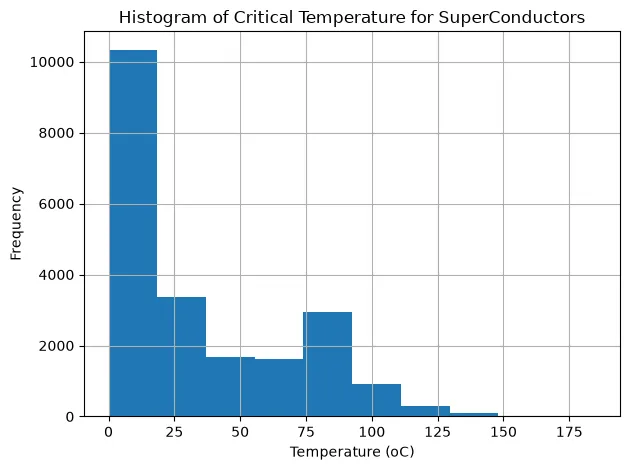 Figure 3: Histogram of the target variable
 critical_temp, showing a pronounced right skew.
To address this, a Box-Cox power transformation was applied to the target variable. After transformation, the distribution became approximately symmetric and bell-shaped — much closer to the normal distribution assumption required by linear regression.
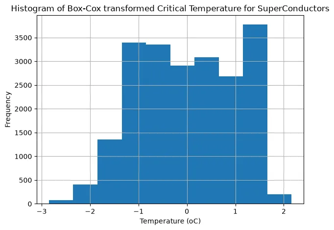 Figure 4: After Box-Cox transformation, the target distribution is approximately normal.
Feature Distributions
Histograms of all 81 predictors in train.csv were plotted on a 9×9 grid, color-coded by their statistical aggregation type:
| Color | Aggregation Type |
|---|---|
| Cyan | mean |
| Green | weighted mean |
| Blue | geometric mean |
| Red | standard deviation |
| Orange | weighted std |
| Purple | entropy |
| Yellow | weighted entropy |
| Olive | range |
| Brown | weighted range |
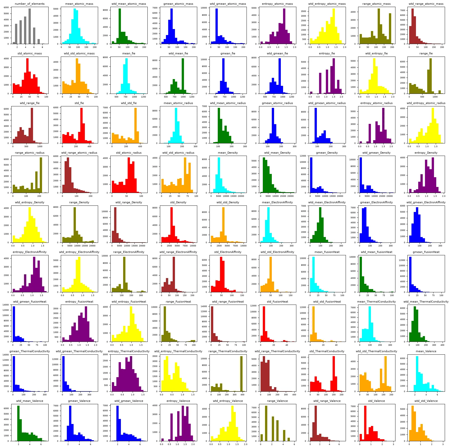 Figure 5: Histograms of all 81 predictors, color-coded by statistical aggregation type. Notice how features within each physical property group share similar distributional shapes.
This visualization revealed that features within the same physical property group (e.g., all 10 aggregations of atomic_mass) tend to have similar distributional shapes, hinting at high inter-feature correlation within groups.
Correlation Analysis
A Pearson correlation heatmap of all 81 predictors confirmed severe multicollinearity. Block-diagonal patterns were clearly visible, indicating that the 10 statistical aggregations within each physical property group are highly correlated with one another.
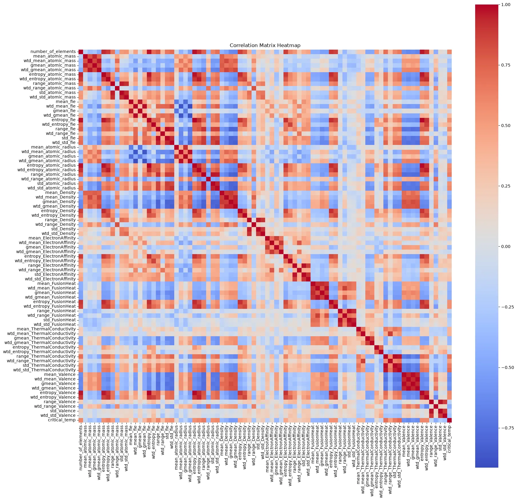 Figure 6: Pearson correlation heatmap for the 81 predictors in
 train.csv. The prominent block-diagonal structure reveals severe multicollinearity within each physical property group.
A separate correlation heatmap of the elemental composition features (from unique_m.csv) showed a more sparse correlation structure, as elemental presence tends to be more independent across compounds.
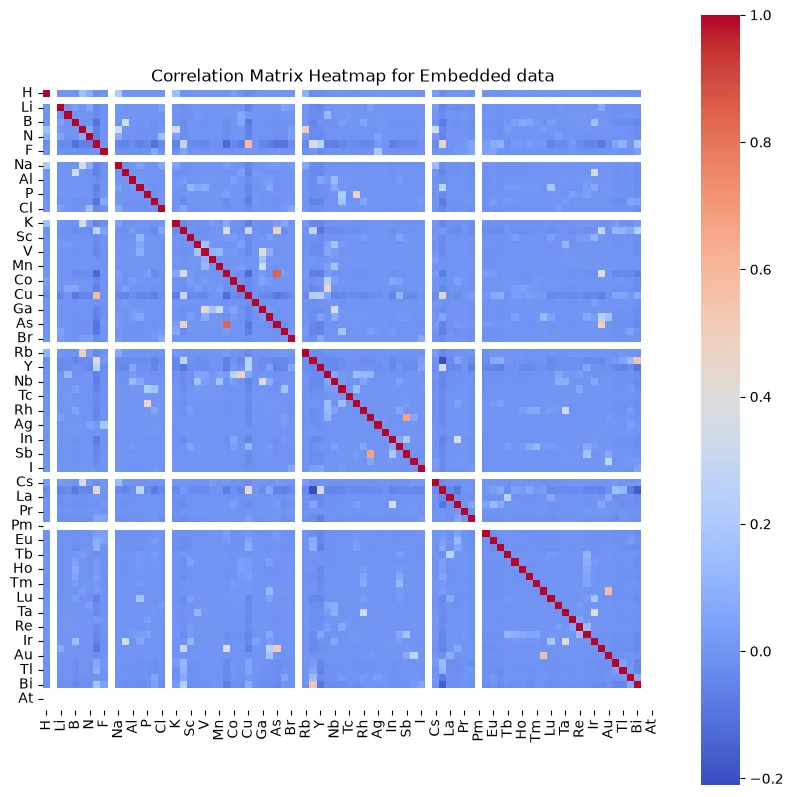 Figure 7: Pearson correlation heatmap for the elemental composition features in
 unique_m.csv, showing a much sparser correlation structure.
Variance Inflation Factor (VIF) Analysis
To quantify multicollinearity, the Variance Inflation Factor (VIF) was computed for every predictor. VIF measures how much the variance of a regression coefficient is inflated due to correlation with other predictors.
| VIF Range | Interpretation |
|---|---|
| 1 – 2 | Very low collinearity; usually no concern |
| 2 – 5 | Moderate; often acceptable |
| 5 – 10 | High; coefficients may be unstable |
| > 10 | Very serious multicollinearity |
Initial VIF Results (All 81 Features)
The initial VIF analysis revealed extremely high VIF values across the board. For example:
| Feature | VIF |
|---|---|
wtd_mean_atomic_mass | 818.37 |
wtd_gmean_atomic_mass | 879.86 |
mean_atomic_mass | 414.28 |
gmean_atomic_mass | 444.20 |
wtd_entropy_Valence | 307.31 |
These values are well above the threshold of 10, confirming that using all 81 features simultaneously in an ordinary linear regression would produce highly unstable coefficient estimates.
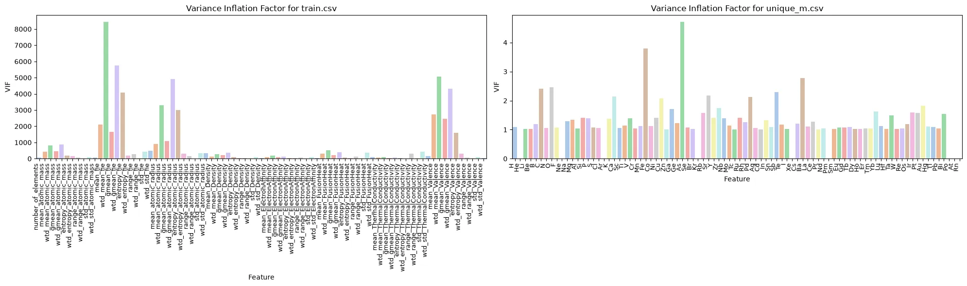 Figure 8: VIF bar plots for
 train.csv features (left) and unique_m.csv features (right) before feature reduction. Most train.csv features exhibit VIF values far exceeding 10.
VIF After Feature Selection
By retaining only one representative aggregation per physical property group (e.g., keeping wtd_range_atomic_mass while dropping the other 9 aggregations of atomic mass), the predictor set was reduced to just 10 features. The VIF values dropped dramatically to acceptable levels:
| Feature | VIF |
|---|---|
number_of_elements | 2.05 |
wtd_range_atomic_mass | 3.95 |
wtd_range_fie | 1.35 |
wtd_range_atomic_radius | 2.20 |
wtd_range_Density | 3.49 |
mean_ElectronAffinity | 1.10 |
mean_FusionHeat | 1.45 |
mean_ThermalConductivity | 1.28 |
wtd_std_Valence | 1.44 |
critical_temp | 2.17 |
All VIF values are now below 5, confirming that this reduced feature set is free of problematic multicollinearity.
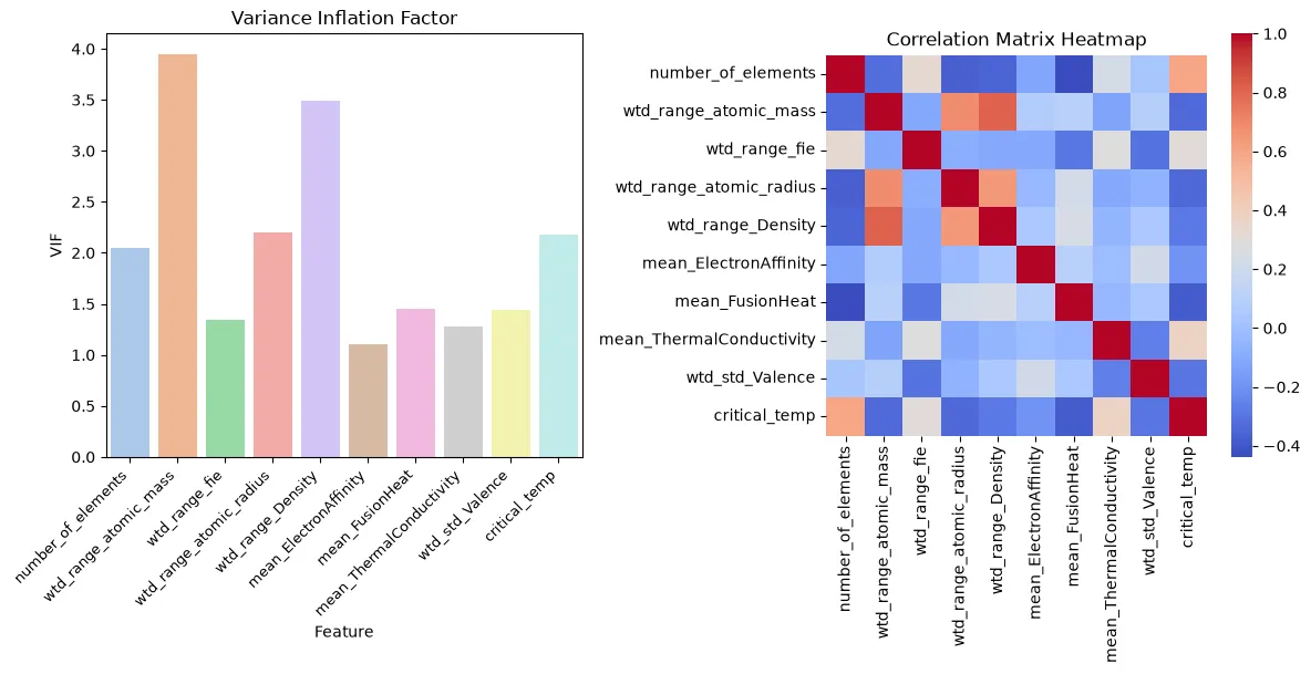 Figure 9: After reducing to one aggregation per group, all VIF values fall well below 5, eliminating multicollinearity concerns.
However, since the purpose of this study is to evaluate regularization methods (which are specifically designed to handle multicollinearity), we proceeded to modeling using all available predictors rather than this reduced set.
Modeling Strategy
Data Preparation
- Feature combination: The scaled
train.csvfeatures (81 predictors) were merged with the unscaled elemental composition features fromunique_m.csv(86 element columns), producing a combined predictor matrix of 167 features. - Scaling:
StandardScalerwas applied to thetrain.csvfeatures to standardize them (zero mean, unit variance). The elemental composition features were left unscaled, as they represent raw counts/proportions. - Train-test split: An 80/20 split was used (
random_state=1234) with shuffling. - Cross-validation: 5-fold cross-validation (
KFold,shuffle=True,random_state=1234) was used for hyperparameter tuning. - Target transformation: For Ridge Regression, the target variable was Box-Cox transformed to correct the right skew. For Lasso Regression, the raw target was used directly.
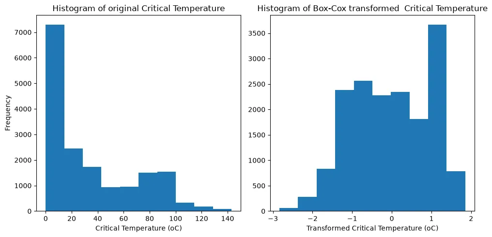 Figure 10: Side-by-side histograms of the training target before (left) and after (right) Box-Cox transformation, showing the skew correction applied for Ridge regression.
Understanding Regularization
In ordinary least squares (OLS) regression, the model minimizes only the sum of squared residuals. When predictors are highly correlated (as in our case with 167 features), OLS coefficients become unstable and can take on very large values.
Regularization adds a penalty term to the loss function that discourages large coefficients:
-
Ridge (L2): Adds a penalty proportional to the sum of squared coefficients ((\alpha \sum \beta_j^2)). This shrinks coefficients toward zero but rarely sets any exactly to zero.
-
Lasso (L1): Adds a penalty proportional to the sum of absolute coefficients ((\alpha \sum |\beta_j|)). This can shrink some coefficients exactly to zero, effectively performing automatic feature selection.
The regularization strength (\alpha) controls the trade-off between fitting the data and keeping coefficients small. Both RidgeCV and LassoCV select the optimal (\alpha) via cross-validation.
Results
Ridge Regression (L2 Regularization)
Ridge regression was trained on the Box-Cox-transformed target using RidgeCV with alpha values searched over np.logspace(-5, 5, 11).
Performance:
| Metric | Value |
|---|---|
| Best CV Score (neg. MSE) | -0.1038 |
| Test-set R² | 0.915 |
| Test-set MSE | 103.53 |
The model explains approximately 91.5% of the variance in the critical temperature on the held-out test set, which is a strong result.
Top 10 Most Important Features (by absolute coefficient):
| Rank | Feature | Coefficient | |Coefficient| |
|---|---|---|---|
| 1 | critical_temp (from df2) | 0.707 | 0.707 |
| 2 | number_of_elements | 0.152 | 0.152 |
| 3 | wtd_range_Density | -0.086 | 0.086 |
| 4 | Ce (Cerium) | -0.066 | 0.066 |
| 5 | In (Indium) | -0.061 | 0.061 |
| 6 | Ag (Silver) | -0.060 | 0.060 |
| 7 | Fe (Iron) | 0.057 | 0.057 |
| 8 | Ca (Calcium) | -0.053 | 0.053 |
| 9 | Zn (Zinc) | -0.050 | 0.050 |
| 10 | mean_ElectronAffinity | -0.047 | 0.047 |
Key observations:
- The
critical_tempfeature from the elemental composition dataset (unique_m.csv) dominates with the largest coefficient, suggesting data leakage (discussed further below). number_of_elementsis the second most influential feature, indicating that the complexity of the compound plays a significant role.- Several individual elements (Ce, In, Ag, Fe, Ca, Zn) appear in the top 10, suggesting that specific elemental presence strongly influences superconducting behavior.
- Ridge regression retains all 167 features with non-zero coefficients, distributing the predictive weight broadly.
Lasso Regression (L1 Regularization)
Lasso regression was trained on the raw (untransformed) target using LassoCV with automatic alpha selection.
Performance:
| Metric | Value |
|---|---|
| Optimal Alpha | 0.183 |
| Test-set R² | 1.000 |
| Test-set MSE | 0.040 |
The model achieves a near-perfect R² of 1.0 — an unusually high value that warrants careful scrutiny.
Top 10 Features (by absolute coefficient):
| Rank | Feature | Coefficient |
|---|---|---|
| 1 | critical_temp (from df2) | 34.023 |
| 2 | O (Oxygen) | 0.022 |
| 3–10 | All other features | 0.000 |
Key observations:
- Lasso’s L1 penalty shrinks all but 2 features to exactly zero, performing aggressive feature selection.
- The
critical_tempfeature fromunique_m.csvabsorbs nearly all the predictive power with a coefficient of ~34. - Only
O(Oxygen) retains a tiny non-zero coefficient (0.022), likely reflecting the prevalence of oxide-based superconductors (cuprates) in the dataset.
Lasso Regularization Path
The Lasso path plot illustrates how coefficients evolve as the regularization parameter (\alpha) decreases (less regularization). As (\alpha) shrinks, more features enter the model with non-zero coefficients. Conversely, at higher (\alpha) values, most coefficients are driven to zero. The accompanying RMSE curve shows that model error initially decreases rapidly as key features enter the model, then plateaus once the most important predictors have been included.
Discussion: The Data Leakage Issue
A critical finding in this analysis is the presence of data leakage. Both the train.csv and unique_m.csv datasets contain a critical_temp column. When these datasets are merged for modeling, the critical_temp from unique_m.csv becomes one of the predictor variables — but it is essentially the same variable we are trying to predict.
This explains:
- Why Lasso achieves R² ≈ 1.0: The model simply learns that
critical_temp(predictor) ≈critical_temp(target), with a coefficient of ~34 that rescales the Box-Cox / raw values. - Why Lasso zeroes out all other features: When the target is directly available as a predictor, no other feature adds meaningful information.
- Why Ridge also ranks
critical_tempas the top feature: Even though Ridge retains all features, the leaked variable dominates.
In a real-world application, one should drop the critical_temp column from unique_m.csv before merging datasets to avoid this leakage. The Ridge results without leakage would likely show a lower R² but would represent genuine predictive performance.
Key Takeaways
-
Multicollinearity is pervasive in engineered feature sets. When the same physical property is summarized through 10 different statistical aggregations, these summaries are inevitably correlated. VIF analysis is a simple and effective diagnostic tool.
-
Regularization handles multicollinearity gracefully. Rather than manually selecting one feature per group (which the VIF analysis demonstrated could reduce 81 features to 10 with acceptable VIFs), Ridge and Lasso automatically manage correlated predictors through their penalty terms.
-
Ridge vs. Lasso serve different purposes:
- Ridge is ideal when you believe all features contribute and you want stable coefficient estimates. It shrinks coefficients but retains all of them.
- Lasso is ideal for feature selection. It produces sparse models by driving irrelevant coefficients exactly to zero, making results more interpretable.
-
Data leakage is a common pitfall in machine learning pipelines. When merging multiple data sources, always verify that no form of the target variable appears among the predictors. A model with suspiciously perfect performance (R² ≈ 1.0) should raise a red flag.
-
Box-Cox transformation can be a valuable preprocessing step when the target variable is right-skewed. It helps linear models meet the normality assumption, potentially improving both stability and performance.
Conclusion
This case study demonstrates the practical application of L1 and L2 regularization to a real-world materials science problem: predicting the critical temperature of superconductors. Through exploratory data analysis, VIF diagnostics, and model comparison, we showed that regularized regression methods can effectively handle high-dimensional, multicollinear data.
The Ridge model achieved a strong R² of 0.915 on the test set when using a Box-Cox-transformed target, while the Lasso model revealed, through its aggressive feature selection, that the merged dataset contained data leakage via a duplicated target variable. This finding underscores the importance of careful data validation before model training.
For future work, removing the leaked feature and comparing model performance on the clean dataset would provide a more honest assessment of predictive accuracy. Additionally, exploring non-linear models (e.g., Random Forests, Gradient Boosting) may capture complex relationships between elemental properties and superconducting behavior that linear models miss.
This analysis was conducted using Python with scikit-learn, pandas, NumPy, seaborn, matplotlib, and statsmodels.